Introduction

RoboDK CAM adds CAM software features to RoboDK software. RoboDK CAM supports different manufacturing processes for robots, CNCs and custom mechanisms in RoboDK. These manufacturing processes include milling, turning, cutting, additive manufacturing, and more. RoboDK CAM also allows you to simulate material removal.

The main controls of RoboDK CAM are located on the toolbar that appears after installing the Add-in:

Quick start tutorial

This quick start guide provides general overview of RoboDK CAM features, and it will help you get familiar with RoboDK CAM for machining.

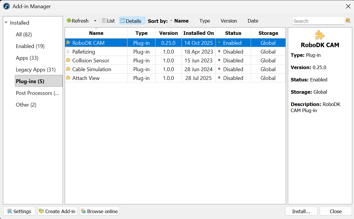
Install RoboDK CAM

You can install RoboDK CAM as an Add-in by opening the RoboDK CAM RDKP package file using RoboDK. Make sure to use the latest version of RoboDK.

RoboDK CAM is only supported on Windows.

Cutter Tool Library

The Cutter Tool Library is the collection of machine cutting tools, or end mills. These tools or cutters are what is attached to the robot main tool (e.g. spindle).

Select CAM - Cutter Tool Library or the corresponding icon on the CAM toolbar to show the library of cutters.

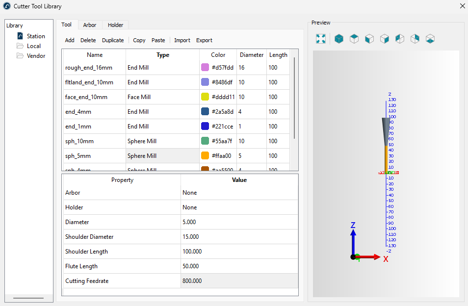
The library window contains three tabs for specifying tools, arbors and holders in tabular form.

If your RoboDK station already contains any robot tools (cutters), they will be displayed in the Cutter Tool Library window. If there are no cutters in the station, you can create them directly in the Cutter Tool Library window using the Add button on the Tool tab.

At the top of the Tool tab, it is necessary to set the tool type. Here, you may also rename the tool or set the color of the cutting edge. To change the corresponding fields, double-click.

At the bottom of the Tool tab, the parameters of the current tool are edited. Different sets of parameters are available for different tool types. For example, an end mill has only three main parameters: diameter, shoulder length, flute length and cutting feedrate.

The tool arbors and tool holders are defined in the corresponding tabs of the Cutter Tool Library window.

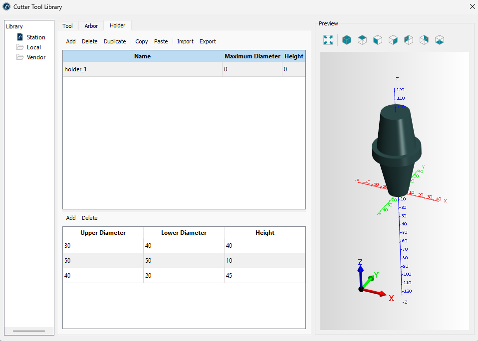
A tool arbor or holder is conventionally represented by a set of cones drawn together. The lower part of the Arbor or Holder tab allows you to specify geometric parameters of cones that make up an arbor or a holder respectively. Several tools can use the same holder or arbor at the same time.

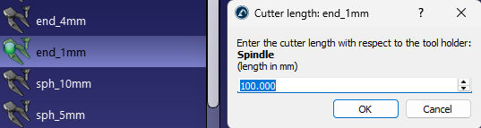
A robot tool with cutting capability is also a Cutter in RoboDK. When you have a cutter, you can ajust the TCP along the Z axis of the holder:

CAM Project

On the RoboDK CAM toolbar, you can select the machining strategy that is suitable for your task.

After selecting the required strategy, the CAM project will be created automatically.

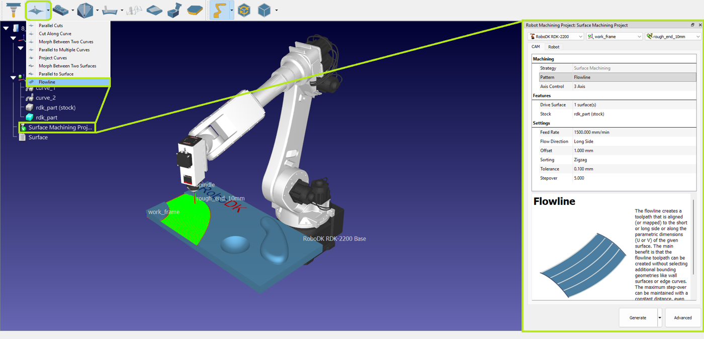
CAM settings

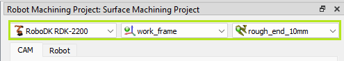
The CAM Project settings window consists of a top section and the CAM and Robot tabs. The robot, reference frame, and cutter are selected in the top section of the window. By default, the active elements at the time of CAM project creation are selected.

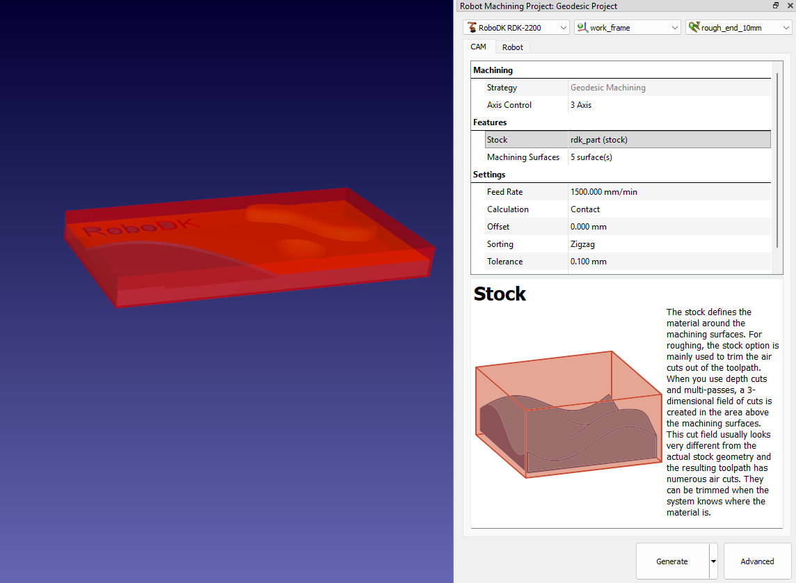
CAM tab

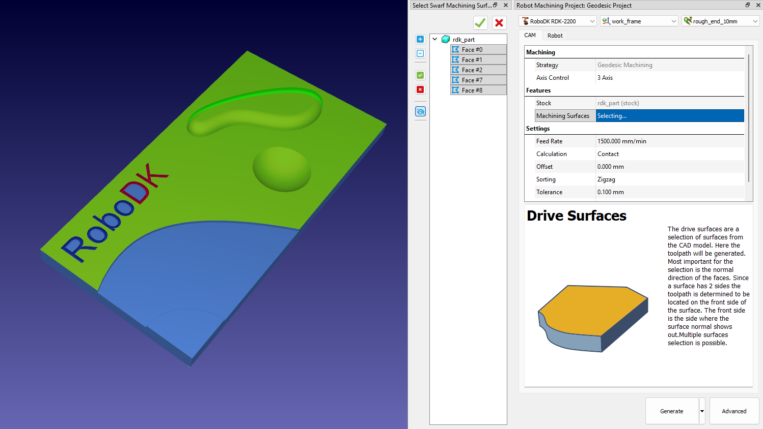
The CAM tab from the CAM project menu contains the machining settings and other strategy settings described in this section.

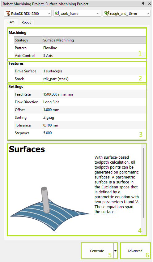
1.Machining settings – indicates selected strategy group and allows to switch between patterns. Additionally, you can select the axes control mode.

2.Features settings – indicates the selected features of the part and stock. This selection is mandatory for calculating the toolpath.

3.Strategy specific settings.

4.Tip – appears when clicking on parameters.

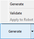
5.Toolpath generation button – calculates the toolpath and applies it to the selected robot. The Validate and Apply to Robot sub-options allow you to separate the calculation and application actions for complex toolpaths.

6.Advanced strategy settings.

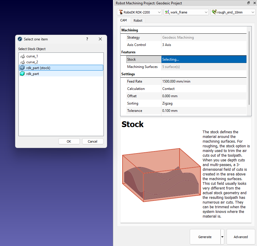
Features selection

In the Features section, you can select the geometric features required for the strategy.Depending on the strategy, you need to select surfaces, curves, or points. The selector tool is launched by double clicking on the features setting line.

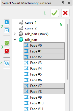
1.Apply selection / Close selector

2.Show tree elements

3.Select all in expanded trees / Clear selection

4.Show / Hide all features

5.Tree view of features

You can check selected geometry features by clicking on selector line.

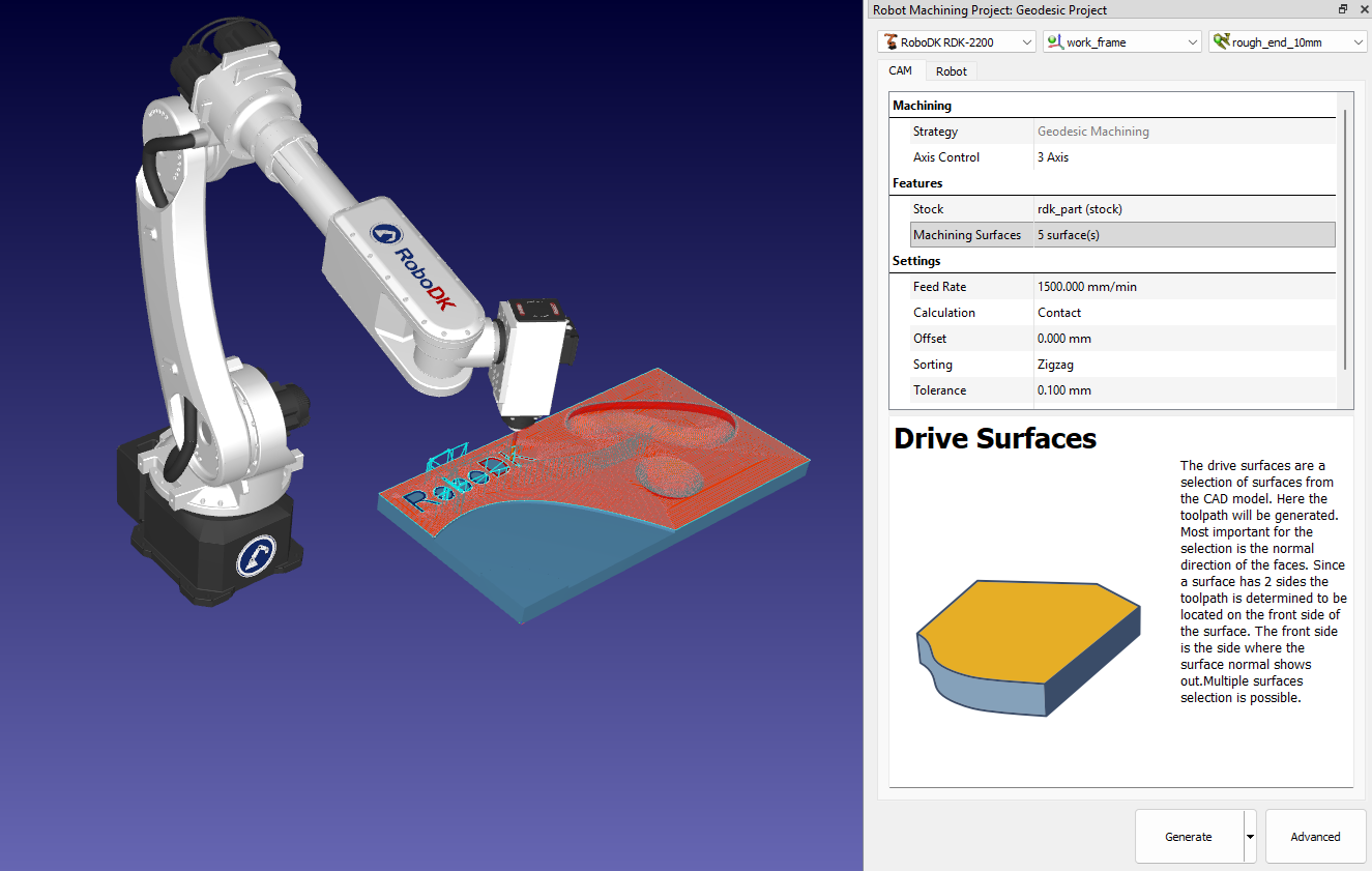
Also, you can specify the model that will be used as a stock.

Robot tab

The Robot tab from the CAM project menu contains the setting related to the robot motion.

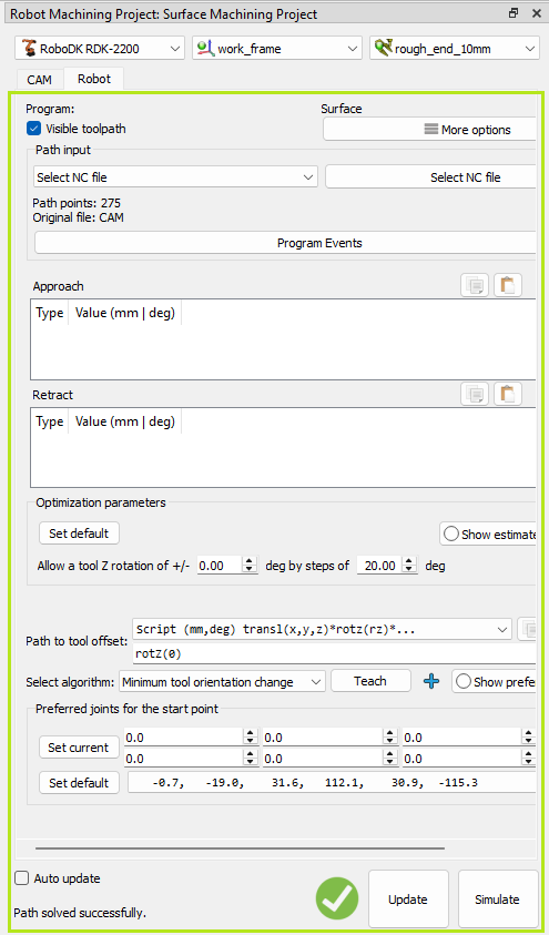
These settings are the same settings you can find in the Robot Machining Project settings of RoboDK.

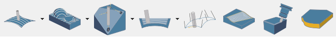
Toolpath strategies

RoboDK CAM allows you to use machining strategies such as surface machining, drilling, roughing, and others. In addition, you can simulate the material removal process.

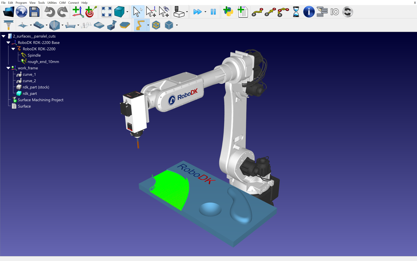
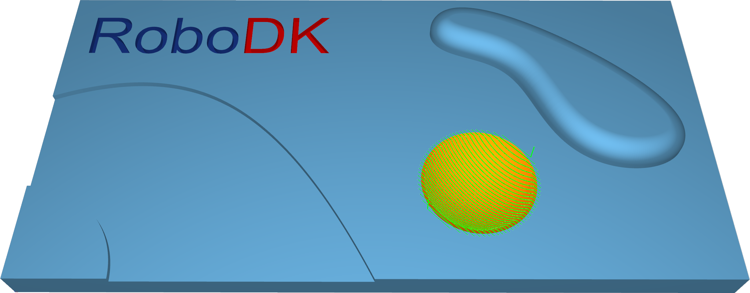
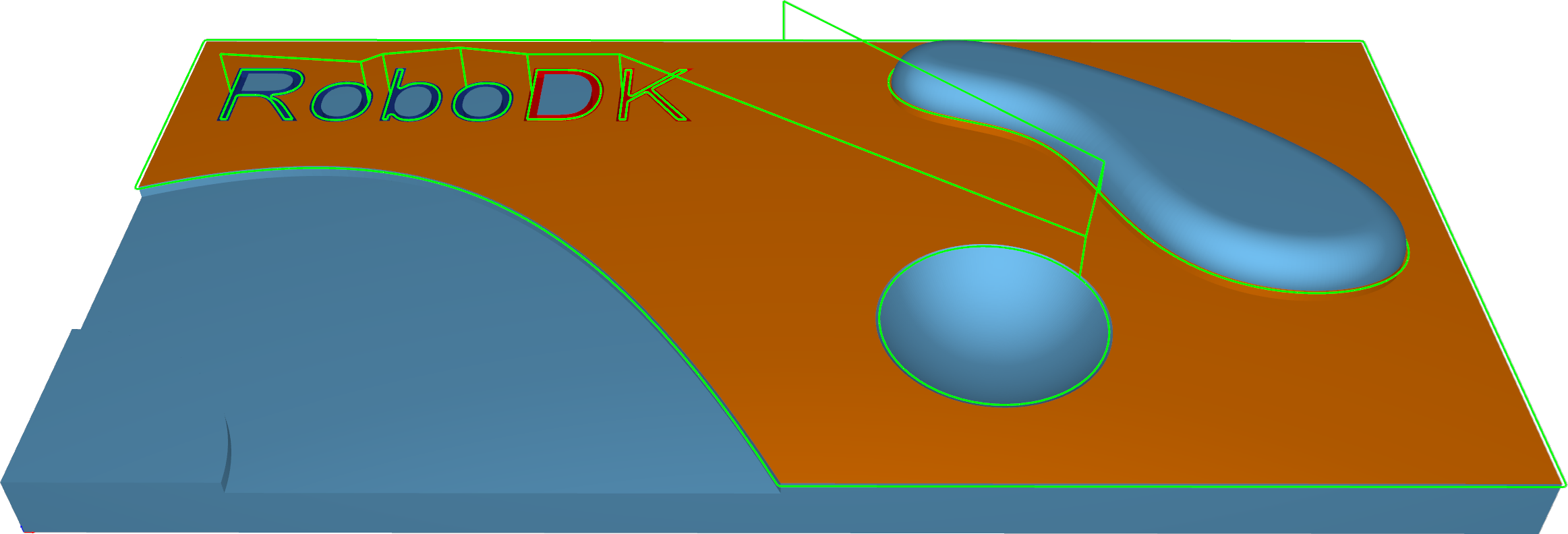
Surfaces–Parallel cuts

The Parallel Cuts option creates a toolpath pattern with parallel slices. The orientation of the slices is defined by two angles: X-Y (which rotates the slices around the Z axis) and Z. Imagine slicing an apple: You can slice it with a knife parallel from top to bottom or from left side to right side. The pictures in the dialog symbolize how to set the desired cutting direction using the angles.

Station: CAM-Surfaces-ParallelCuts.

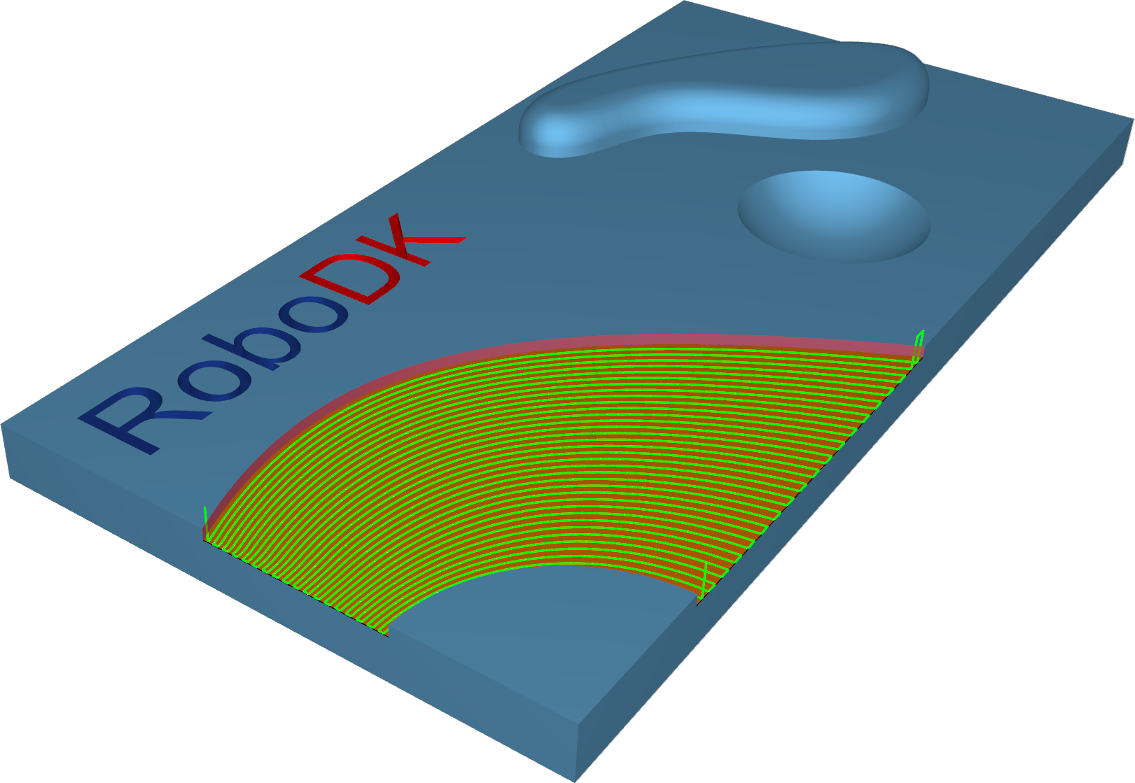
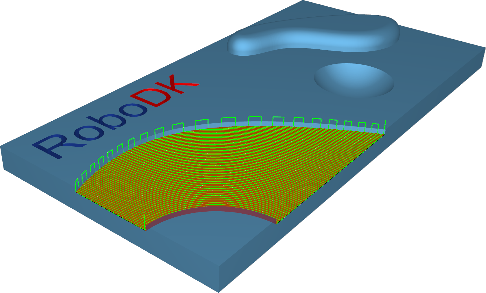
Surfaces–Cuts along curve

The Cuts along curve pattern allows the user to create a toolpath orthogonal to a drive curve. That means that if the selected curve as 'Lead' is not a straight line, the cuts are not parallel to each other.

Station: CAM-Surfaces-CutAlongCurve.

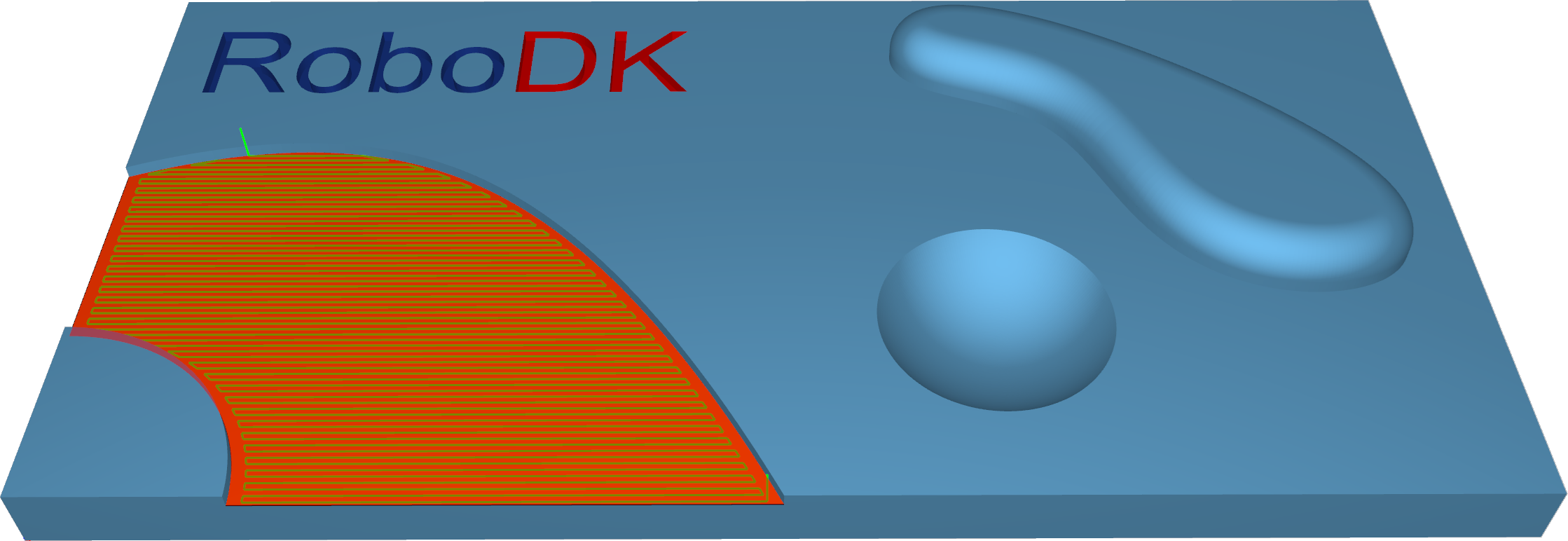
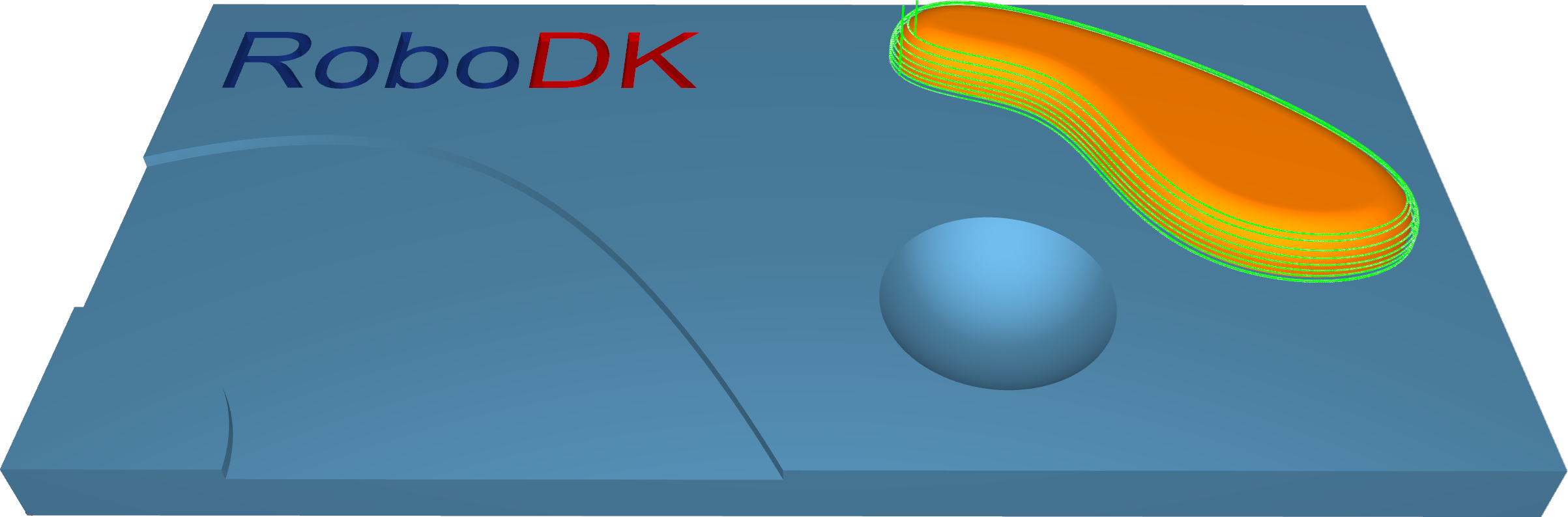
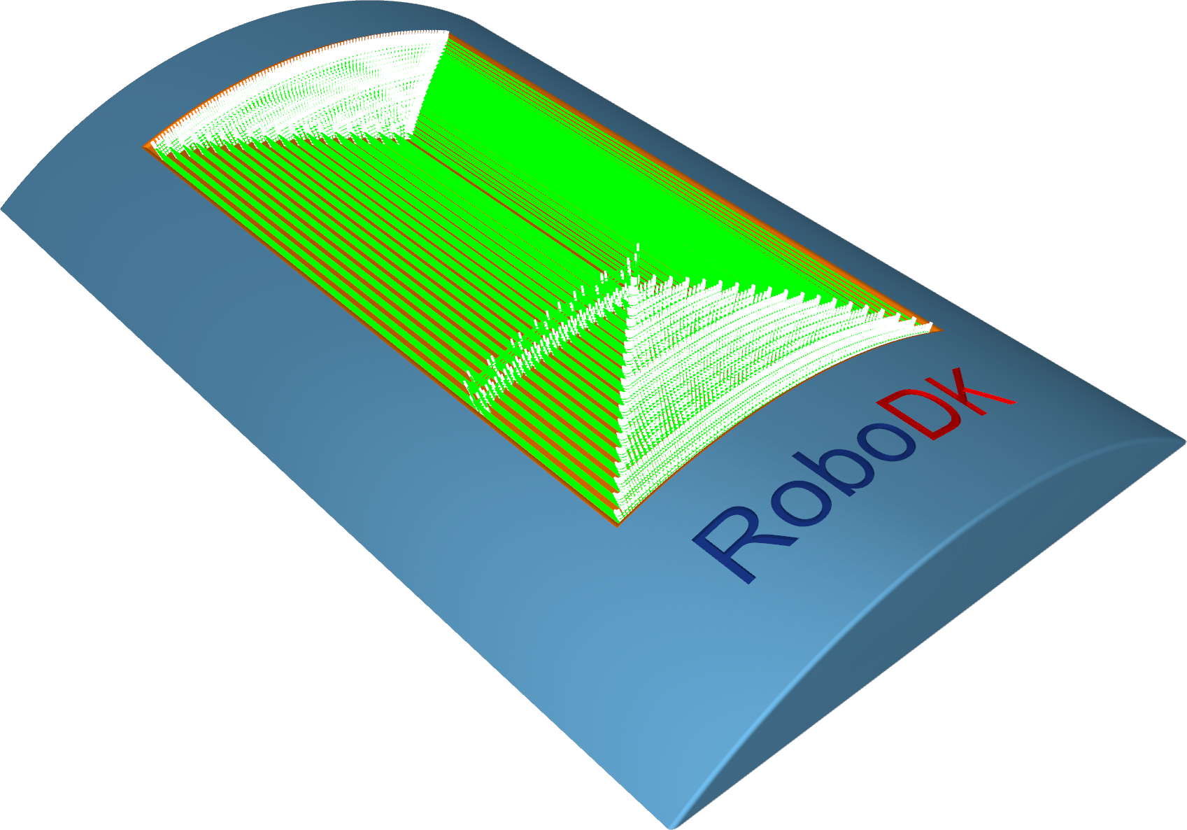
Surfaces–Flowline

The Flowline creates a toolpath that is aligned (or mapped) to the short or long side or along the parametric dimensions (U or V) of the given surface.

The main benefit is that the flowline toolpath can be created without selecting additional bounding geometries like wall surfaces or edge curves. The maximum step-over can be maintained with a constant distance, even if the surface topology is very complex. Also, calculation time is very fast.

Station: CAM-Surfaces-Flowline.

Surfaces–Morph between two curves

This option creates a morph toolpath between two leading curves, input as 'First' and 'Second'. Morph means that the generated toolpath gradually interpolates between the two curves and spreads evenly over the surface.

This option is well-suited for machining steep areas when making molds.

Station: CAM-Surfaces-MorphBetween2Curves.

Surfaces–Morph between two surfaces

This option will create a morph toolpath on the drive surface. The drive surface is enclosed by two check surfaces. Morph means that the generated toolpath is approximated between the check surfaces and evenly spread over the drive surface. Especially the impeller machining with its twisted turbine blades can be machined using this option.

Bi-Tangency - the main advantage is the possibility to compensate the tool to the drive surface and check the surface in the left and right corner of the work piece. All you need to do is to enable the tool radius from (margin) options, which is the distance between the tool center and the surfaces.

Station: CAM-Surfaces-MorphBetween2Surfaces.

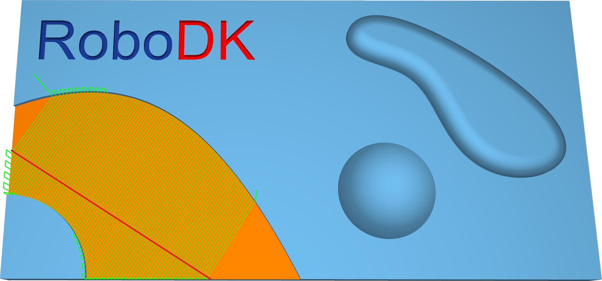
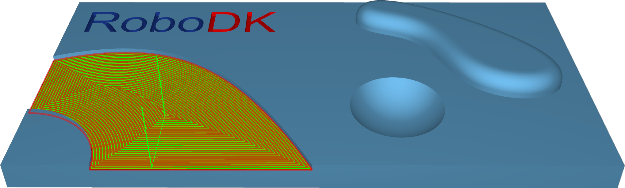
Surfaces–Parallel to multiple curves

The Parallel to curve option will create toolpath segments parallel to the leading curve. The neighboring toolpath segments are parallel to each other. The important point here is that the cuts won't be simply copied next to each other. Every new cut will be an offset of the previous cut.

Important notes:

1.The curve must be located exactly on the surface edge. So, the best curve would be the edge itself. This is very important for toolpath generation. If you don't have a proper leading curve aligned to edge, a wrong toolpath can be generated.

2.For independent curves on the same surface, only the first curve will be used. For more complex models, it means that it is difficult to provide the right leading curve to machine the whole model.

3.For consecutive curves on the same surface, all curves must be joined in a single curve. This step can be performed from any CAD system, or it can be made automatically by the system.

4.For independent curves on the same surface, only the first curve will be used. For more complex models, it means that it is difficult to provide the right leading curve to machine the whole model.

5.Multiple curves selected on independent surfaces will generate different cuts on each surface.

6.The distance between two neighboring toolpath segments is the maximum step-over.

7.You can define a margin to get the exact position where the tool is located at the edge with a certain distance.

8.With the pattern Parallel to multiple curves, it is possible to use multiple curves for multiple surfaces. Each curve will now be used only for the nearest surface.

Station: CAM-Surfaces-Parlallel2MultipleCurves.

Surfaces–Parallel to surface

Parallel to surface will create cuts on your drive surface that are parallel to a leading surface.

Station: CAM-Surfaces-Parallel2Surface.

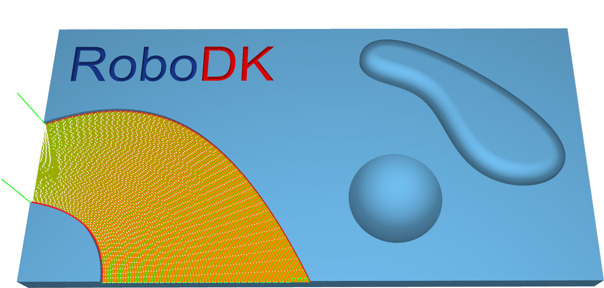
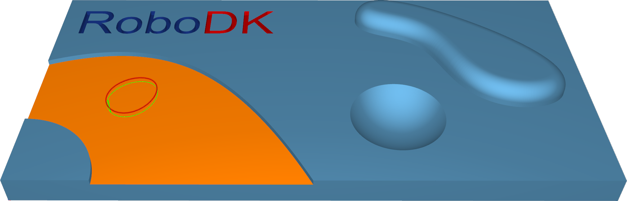
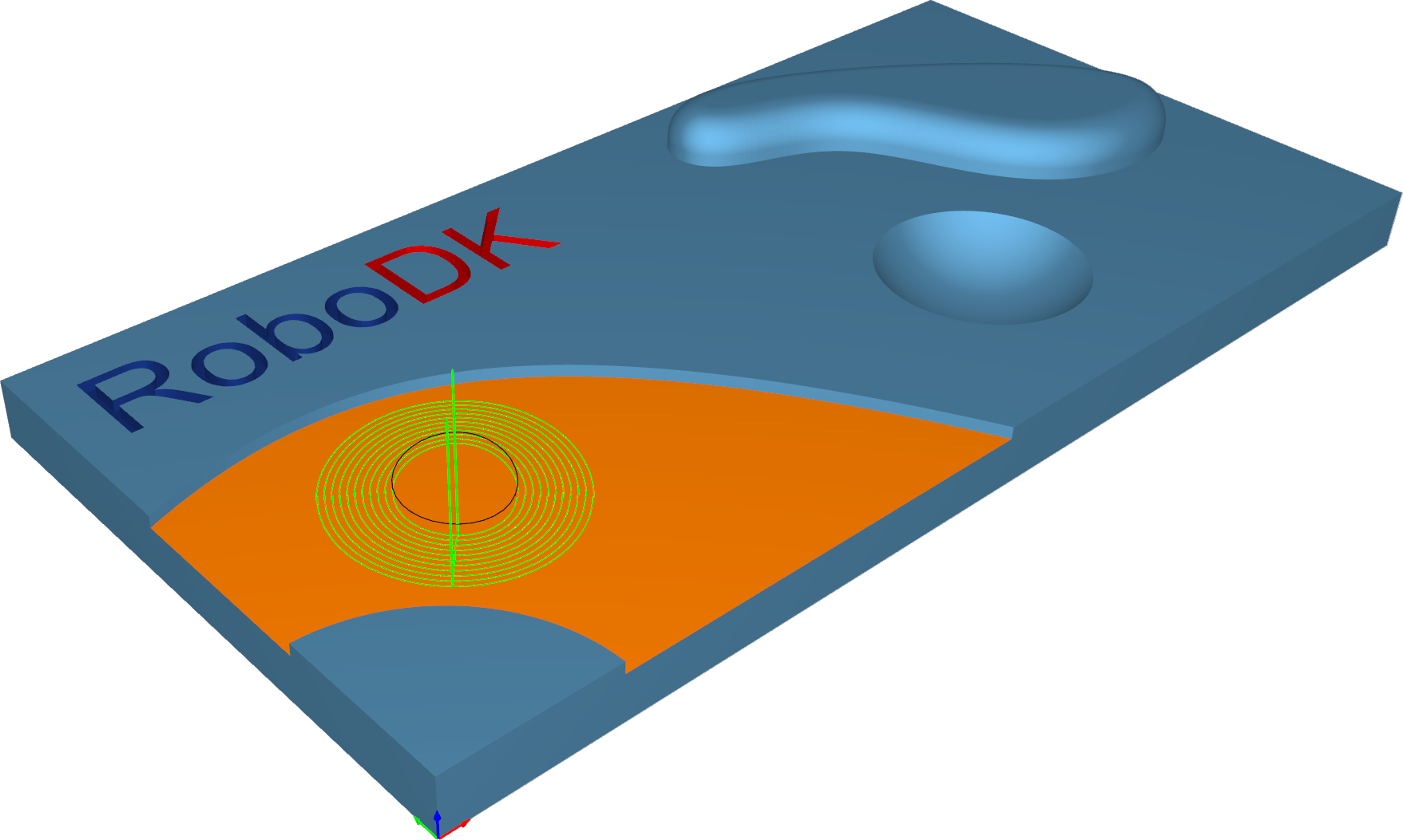
Surfaces–Project curve

With this pattern, either a user-defined curve or a generic pattern can be created. There are 2 2D pattern projections, radial and spiral, and 2 3D curve projections: offset and user-defined.

Station: CAM-Surfaces-ProjectCurve.

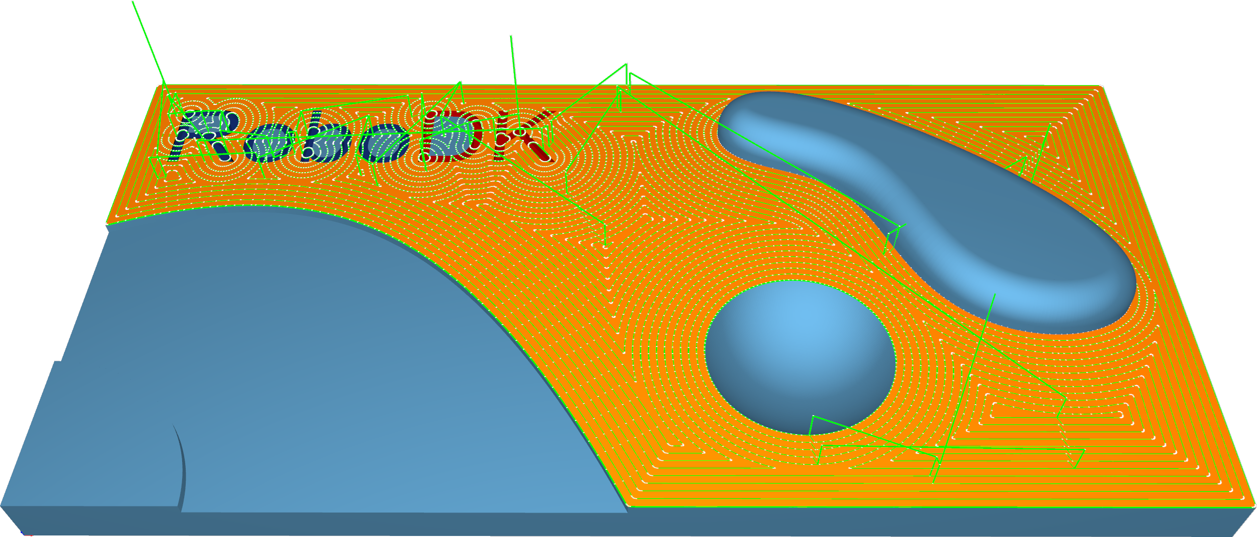
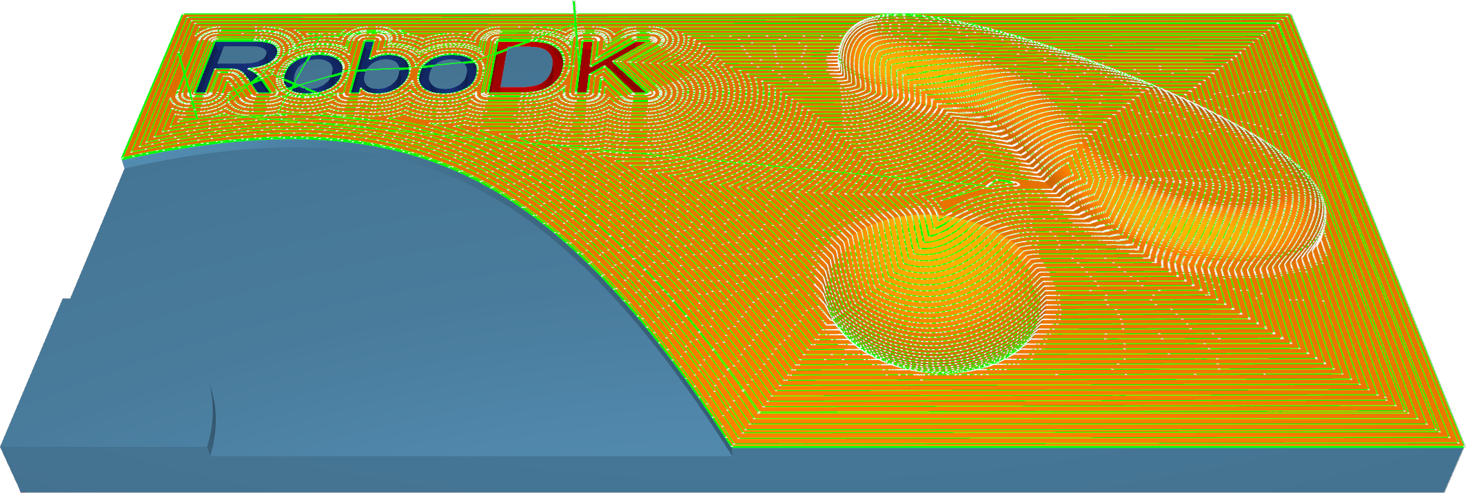
Trimesh–Rough

Roughing is the first stage of machining. This strategy is used to remove large volumes of excess material very quickly and leave a small amount of stock for semi-finishing and finishing strategies. You can use this strategy to create a rough component from a rectangular or core-shaped block.

Toolpath cuts material in successive Z-levels, working from top to down. The 'Depth step' parameter defines the distance between two Z levels. Toolpath is created from model slices and offset outwards. The distance between two offsets is defined by step-over. The toolpath segments are trimmed to block limits. The result is a rough component with a staircase effect over the whole component, which differs from the finished component by a thickness whose value is defined in the offset field.

Station: CAM-Trimesh-Rough.

Trimesh–Parallel cuts

This strategy allows the machining of 3d components with toolpath passes that are parallel to each other relative to axes X and Y. Any desired angle in the XY plane can be set using the 'Machining angle in X,Y' parameter.

This strategy is generally used to semi-finish or finish a component. It is best suited to shallow machine areas.

Station: CAM-Trimesh-ParallelCuts.

Trimesh–Project curve

In the Project curve strategy, a 2d or 3d curve pattern is projected on the triangle mesh to create a toolpath.

Station: CAM-Trimesh-ProjectCurve.

Trimesh–Constant Z

This strategy allows the machining of 3d components with toolpath passes that are parallel to a plane that depends on the machining direction. Imagine a component being sliced from top to bottom.

This strategy is generally used to semi-finish or finish a component. It is best suited to machine steep areas - vertical or near vertical walls of a 3d component.

1.Constant Z + Constant Cusp: This pattern enables you to machine parts consisting of steep and shallow regions in one iteration. Steep regions are machined with the help of Constant Z slices. A constant cusp is applied for shallow area processing. 

2.Constant Z + Parallel Cuts: This pattern makes it possible to machine parts consisting of steep and shallow regions in one iteration. Steep regions are machined with the help of Constant Z slices. Parallel cuts are applied for shallow area processing.

Station: CAM-Trimesh-ConstantZ.

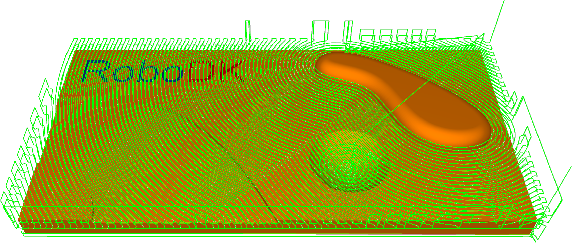
Trimesh–Constant Cusp

This strategy will create an equidistant cut pattern on the machining surfaces. The aim is to have a constant distance between each contour so that the cusps created will have the same height.

This strategy is generally used to semi-finish or finish a component. It is best suited to machine steep as well as shallow areas.

Station: CAM-Trimesh-ConstantCusp.

Trimesh–Flatlands

This strategy is designed to machine true flat areas of 3d components with toolpath passes that are offset segments of the flat area boundary. It is generally used to finish a component. It is best suited to machine large flat areas at multiple Z levels.

Flat areas like parting surfaces can be machined by an endmill or bullnose mill cutter using flatlands machining strategy.

Station: CAM-Trimesh-Flatlands.

Trimesh–Pencil

This strategy is intended to provide fast corners and fillets processing. It can be performed via single- or multi-pencil cuts.

Station: CAM-Trimesh-Pencil.

Trimesh–Trochoidal

The strategy provides sequential part contour machining by trochoidal movements.

Could be applied for cutting out part from the stock material.

Station: CAM-Trimesh-Trochoidal.

Wireframe–5-Axis Profiling

This calculation provides toolpath generation based on wireframe input drive curves. It works without any machining surfaces.

The tool orientation is defined by tilt lines and is perpendicular to the orientation lines. Tilting settings are required, which can be controlled by the tilting options. The tool axis orientations are interpolated between the lines.

Station: CAM-Wireframe-5ax.

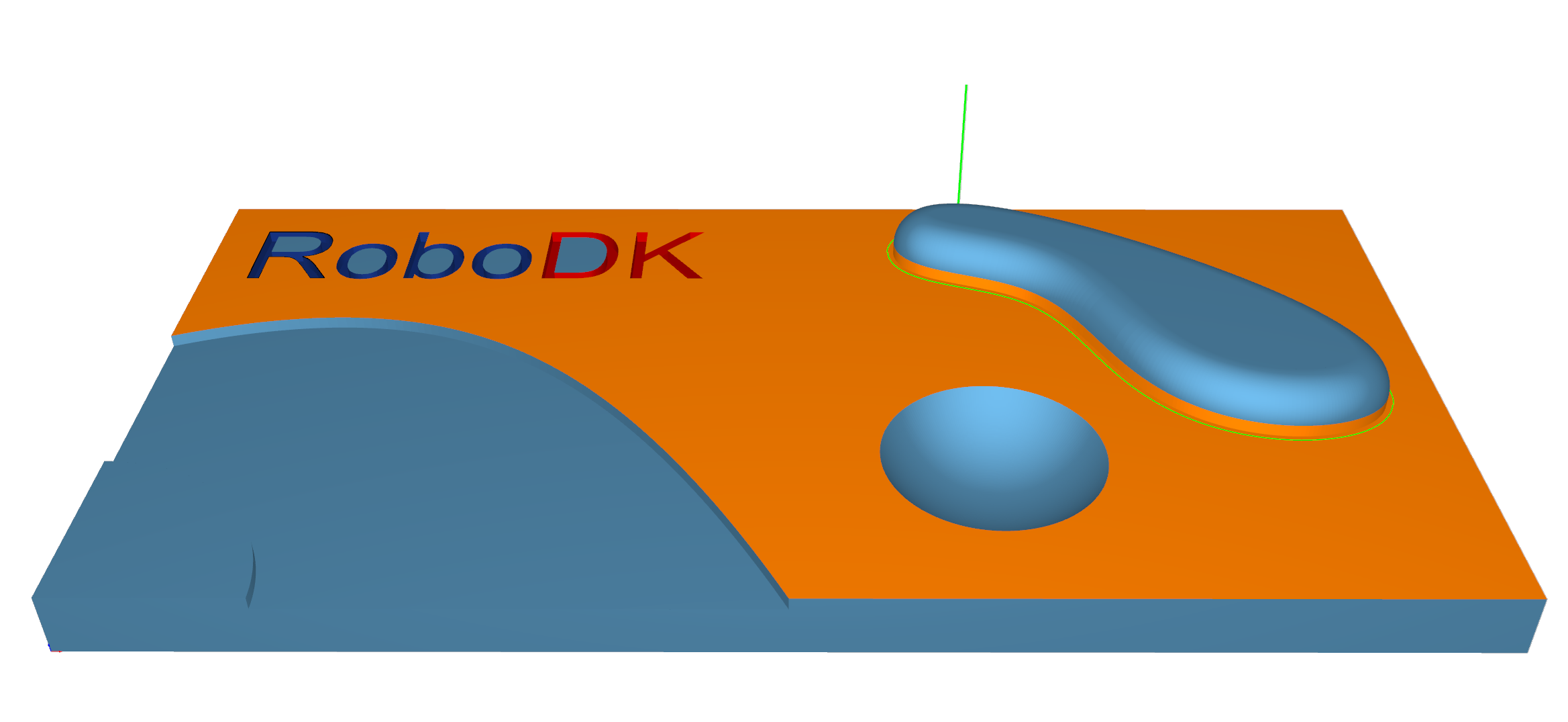
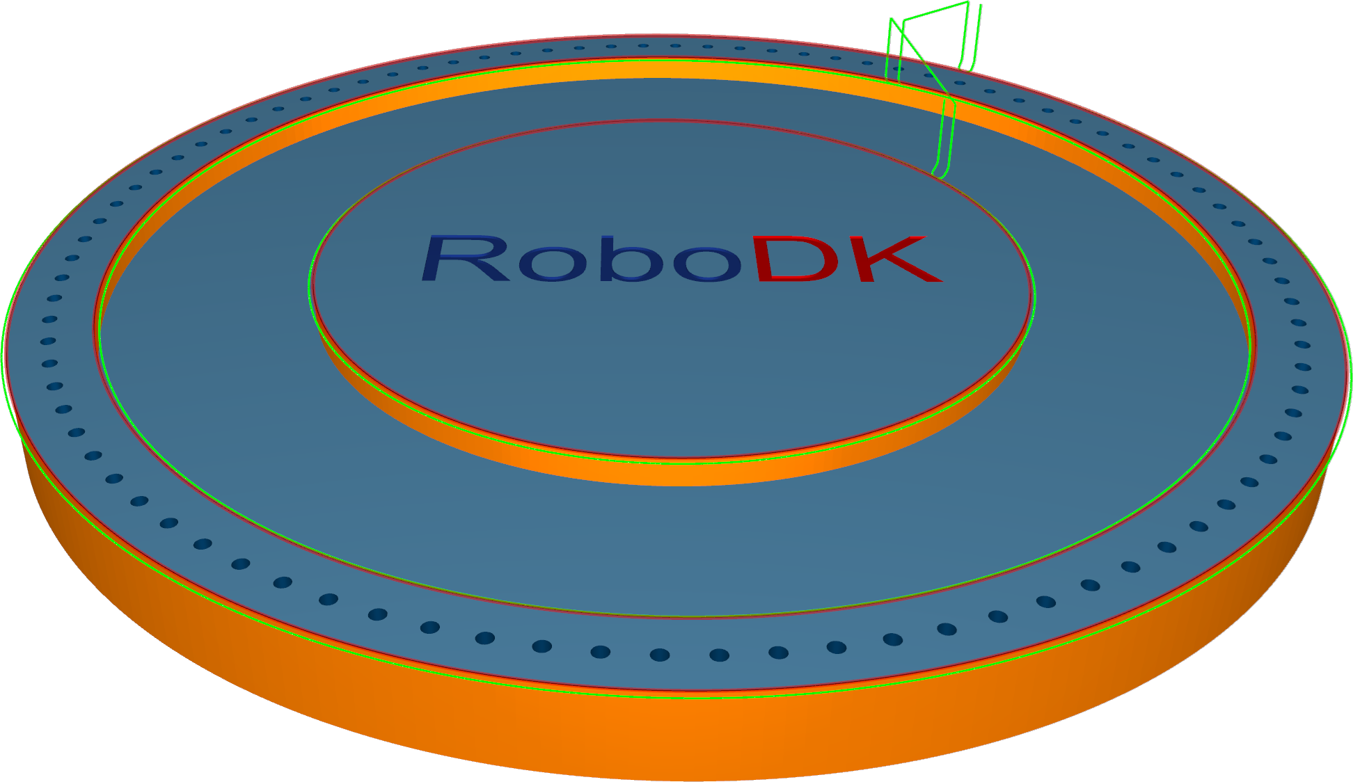
Contouring

Contouring is a highly automated algorithm to create the edge trimming toolpath.

The Contouring calculation strategy is designed for the edge trimming of thin materials. The position of the tool relative to the geometry can be defined by various options, from only a 3-axis output to a more complex 5-axis output with different tool axis orientation options. A key feature of this algorithm is the axial shift where the tool can be engaged with a certain value into the material. The contour can be automated or user-defined.

Station: CAM-Contouring.

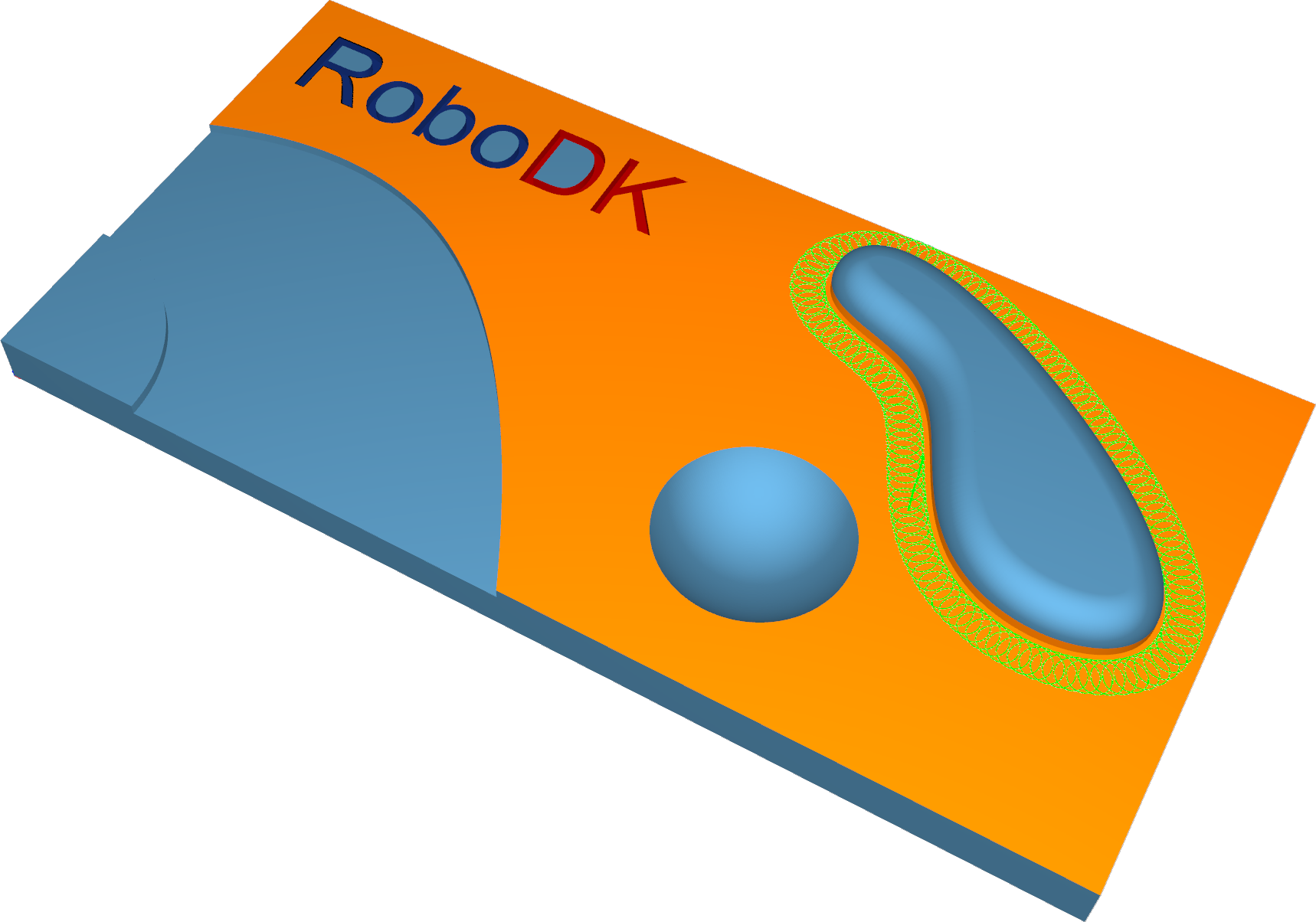
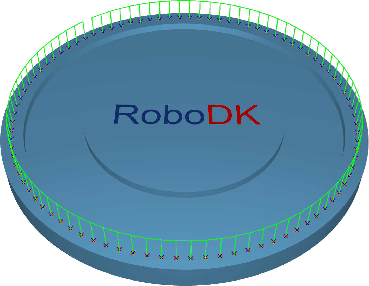
Deburring

The Deburring algorithm creates a deburring toolpath on the outer edges of a part geometry. By default, the orientation of spherical tools relative to the edge is the bi-vector between the two surfaces of that edge. Special tilt settings and other tools adjust the orientation as required.

To detect all the edges, the geometry input (a mesh) must be of good quality.

Station: CAM-Deburring.

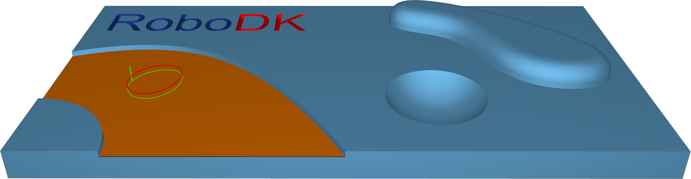
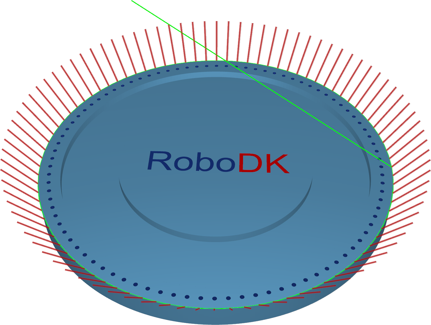
Drilling

The calculation based on drilling points is a very basic drill cycle. It works without any machining surfaces. Drill positions and orientations will be defined either with points or lines.

On surface - with points/lines on the surface, the user must select points/lines that are positioned directly on the surface. The orientation of the tool axis is determined by the surface normal.

Points - For this cycle, the user must select points from the geometry.  The drill cycle starts at the selected points. The orientation must be set up on the Tool axis control tab.

Lines - For this cycle, the user must select lines from the geometry. The lines define the position and orientation of the tool as well as the drill depth.

Station: CAM-Drilling-Points.

Geodesic

Geodesic is a generalization of the concept of a "straight line" mapped onto "curved spaces". Those geodesic distances are used to create patterns that consider the distances on the surface topology.

Geodesic machining provides two modes:

1.The contact point mode supports all tools. The output is similar to the surface-based pattern and does not guarantee a collision-free pattern with the surrounding geometry (e.g., in inner corners).

2.The tool center mode supports ball tools only. The calculation is generated in offset space to avoid collisions with the surrounding geometry.

Station: CAM-Geodesic.

Multiaxis

The multiaxis algorithm creates a multiaxis toolpath that can be used to machine pocket-shaped geometries. The calculation uses STL meshes and IGES geometries as input. The user must specify the floor, wall, and ceiling surfaces, and the system then automatically creates the toolpath.

The Multiaxis Roughing algorithm creates a multiaxis toolpath that can be used to rough out pocket-shaped geometries. The parameters are identical to the triangle, mesh-based roughing cycle, which includes the adaptive roughing feature.

The Multiaxis Floor Finish algorithm creates a multiaxis toolpath for finishing pocket-shaped geometries. Users must specify the part and floor surfaces.

The Multiaxis Wall Finish algorithm creates a multiaxis toolpath that can be used to finish pocket-shaped geometries. The user must specify the floor and wall.

The Multiaxis Rest Finish algorithm creates a multiaxis toolpath for rest finishing pocket-shaped geometries. The user must provide the floor and wall finishing operations as input. The calculation uses containment curves around the unmachined areas, either provided by the user or automatically derived from previous multiaxis machining operations.

The user can choose which areas to machine, and which curves to use as guide curves by selecting one of the following options:

1.Medial axis: The medial axis is used as the drive curve. The main part of the medial axis is calculated from the containment curves.

2.Floor boundary: The boundary of the floor surface is used as the guide curve.

3.Do not machine: Do not machine this area.

Station: CAM-Multiaxis-Roughing.

Material Removal Simulation

The Material Removal Simulation is a dynamic step-by-step visualization of the material removal process. It provides a detailed simulation of how a tool cuts a part or stock, allowing you to observe each stage of the machining process.

You should follow these steps to properly simulate material removal with RoboDK CAM:

1.The cutter must be defined.

2.Link the robot or CNC if there are more than one robot arm in the station.

3.Specify the stock object.

4.Enable cutting simulation. Otherwise, the simulation will run without material removal.

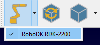
Link the robot

Use the down arrow on the Link Robot button to bring up a menu of available robots and link the simulation to one of them. If the button is in selected state (the robot is linked), pressing it will cause the robot to disconnect from the simulation.

The linking between the robot and the simulation can also be done using the context menu in the station tree.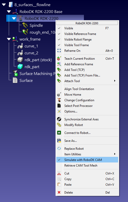

Once the robot is linked to the simulation, any robot movements in the RoboDK window will be repeated by the simulator as tool movements. Regardless of the source of this movement: a RoboDK program, a Python script, or manual movement with a mouse.

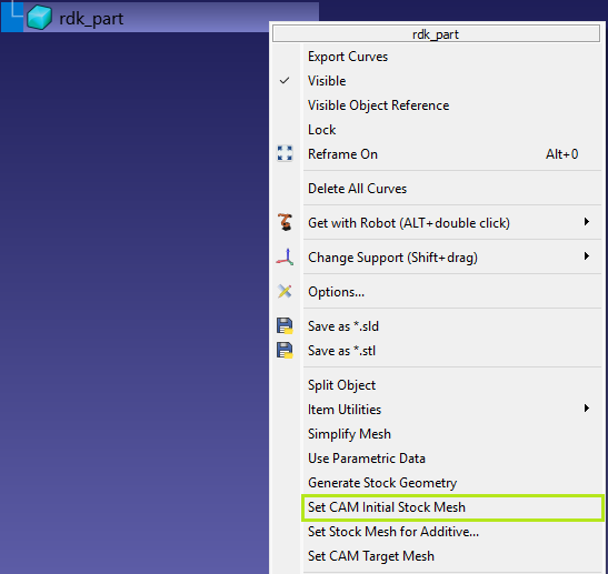
Definition of the stock object

Right-click on the stock object in the RoboDK station tree and select Set CAM Initial Stock Mesh.

Generation of the stock object

Right-click on the stock object in the RoboDK station tree and select Generate Stock Geometry.

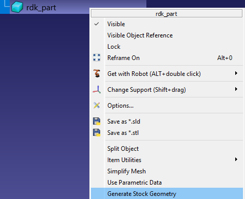
This command will launch the stock creation utility, which uses the original model shape for the generation process.

There are three methods for generating stocks:

1.Bounding box – Box tab

2.Bounding cylinder – Cylinder tab

3.Scaling – From Source Model tab

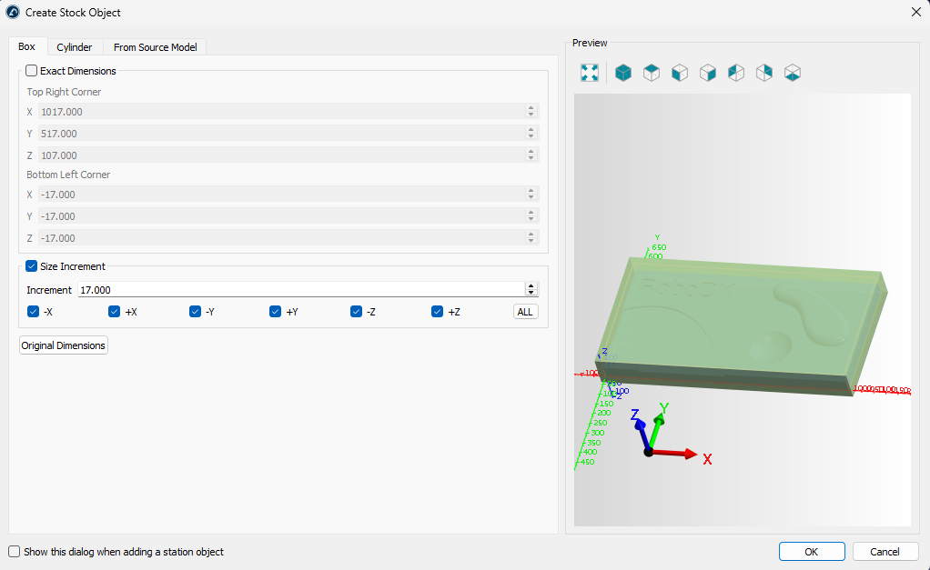
On the Box tab, you can specify the exact dimensions of the bounding box or generate it by extracting (using the Original Dimensions button) and enlarging specific dimensions.

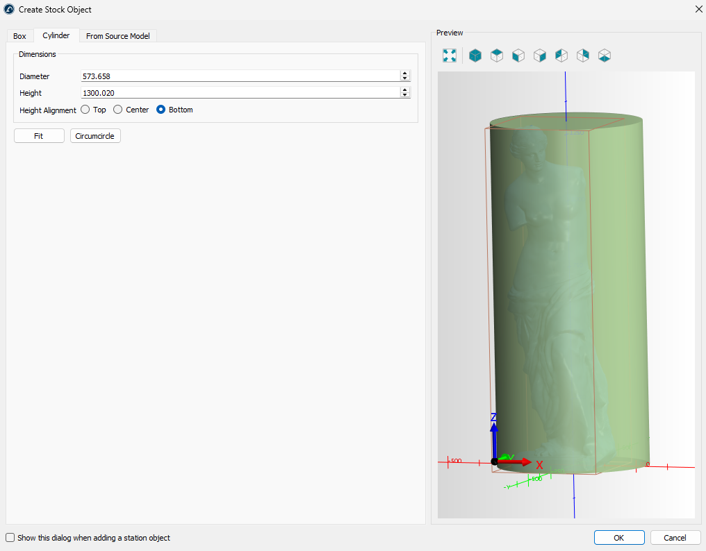
The Cylinder tab allows you to create a stock in the form of a cylinder containing the original model.

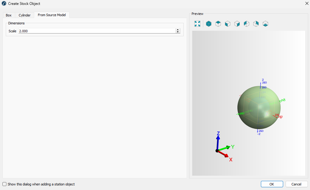
The From Source Model tab allows you to create a stock in the form of a scaled original model.

Stock View

Once the stock definition is complete, the simulation stock model will be displayed on top of the other models in the RoboDK scene. You can control the view of the stock simulation using the Stock View submenu on the toolbar:

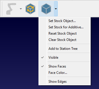
Set Stock Object – define/redefine a stock object.

Set Stock for Additive Object – define/redefine an additive stock object.

Reset Stock Object – revert the stock to its initial state.

Clear Stock Object – delete a stock object.

Add to Station Tree – copy the stock in its current state as as model into the RoboDK station tree.

Visible – stock visibility switch.

Show Faces – show stock faces.

Face Color… – set the default color for the faces.

Show Edges – show stock edges.

Activate material removal simulation

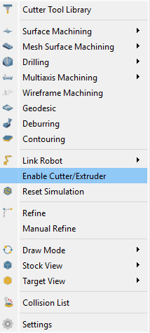
Material removal simulation is activated automatically. However, you can control it manually using the CAM-Enable Cutter/Extruder command.

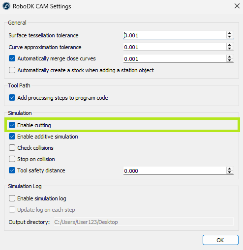
Also, it’s necessary to check if the CAM-Settings-Simulation-Enable cutting setting is active.

Reset Simulation

Simulation reset command reverts the stock to its initial state.

Target View

You can compare the current state of the stock with the target model. To do this, you first need to set the target model using CAM-Target View-Set Target Object, and then apply CAM-Draw Mode-Deviation Map.

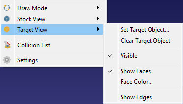
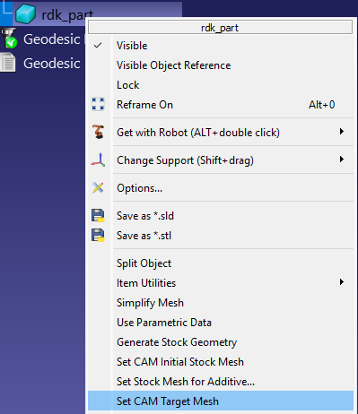
To set the target object, you can also right-click on the model in the station tree and select the Set CAM Target Mesh command.

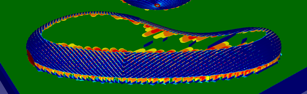
Deviation Map

The deviation map shows the relative difference using a colour scale ranging from green, indicating no difference, to red, indicating the greatest difference.

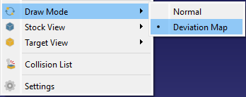
Select CAM-Draw Mode-Deviation Map to show the defiation map.

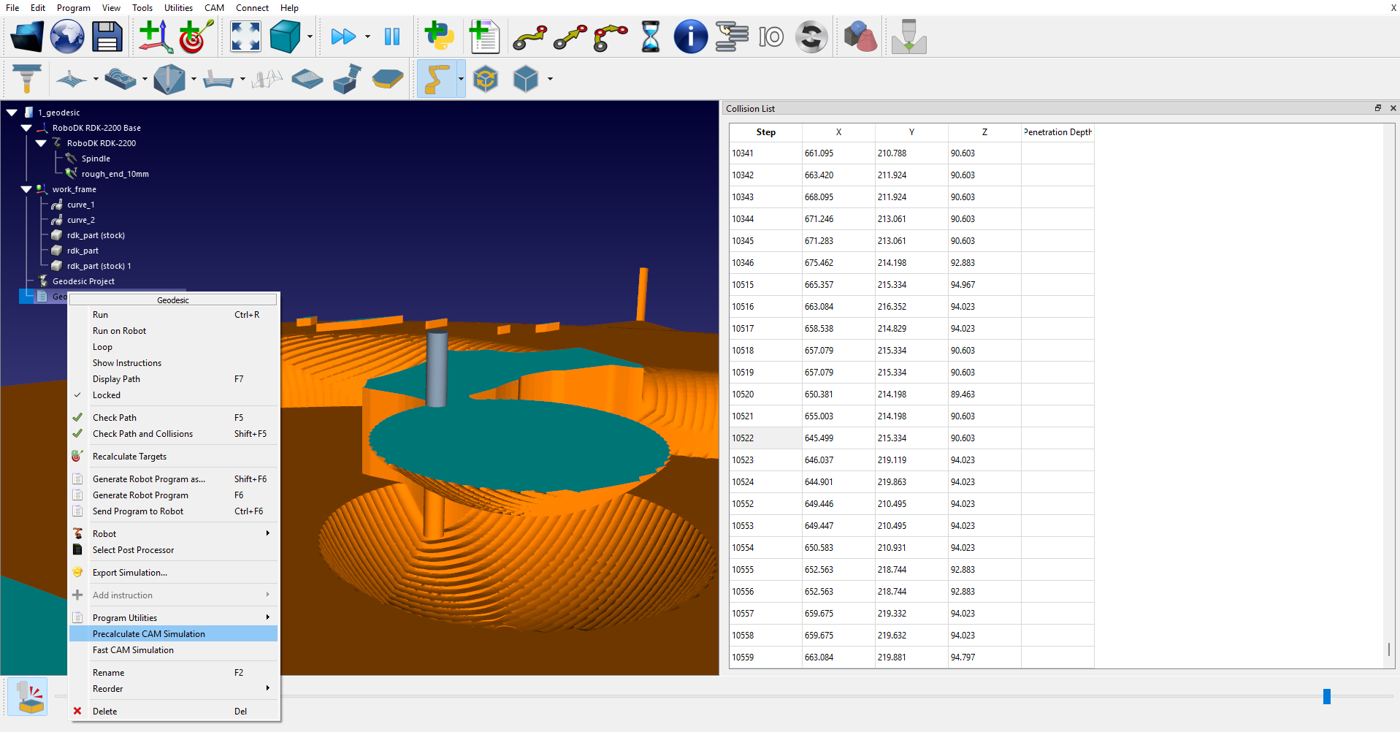
Collision List

The collision list shows the sequence of collisions between the non-cutting parts of the cutter tool (e.g. holder) and the workpiece during machining.

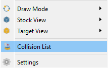
Select CAM-Collision List to show the collision list.

Refine/Manual Refine

With the Refine option enabled, you can obtain higher-quality surface visualization during simulation (this may affect rendering performance).

Using the Manual Refine command, you can improve the visualization of surfaces once after pressing it.

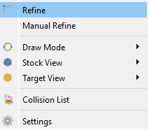
Select CAM-Refine / CAM-Manual Refine to perform the refine operation.

Fast CAM Simulation

You can run a quick simulation of material removal. To do this, right-click on the target program and select the Fast CAM Simulation command.

Settings

By clicking on the CAM-Settings you will be able to adjust the default RoboDK CAM settings.

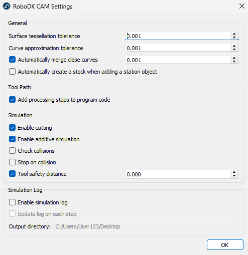
General

The General Settings group includes tolerance settings for model import. In addition, you can enable the Auto Create Stock option, which will display the corresponding dialog box each time you add any model to the station.

Tool Path

The Tool Path settings group includes the Add processing steps to program code option. When this option is enabled, additional information related to the machining process will be added to the generated program.

Simulation

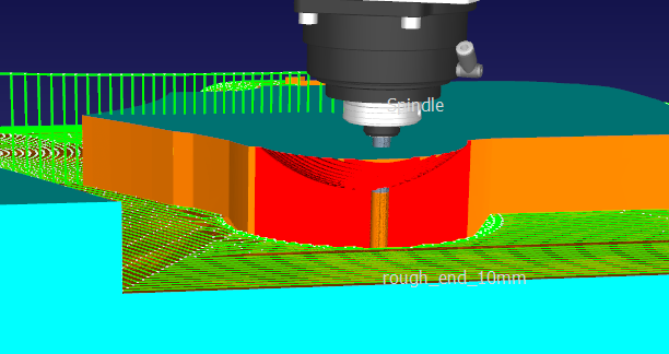
The Simulation settings group includes parameters that enable material removal/addition simulation and collision checking. The Tool Safety Distance parameter can be used to specify an additional distance between the non-cutting parts of the cutter tool and the material. This distance will be taken into account during collision checking.

Collision surfaces will be marked in red.

Log

The Simulation Log settings group includes log parameters that can help investigate simulation-related issues.